Data Pipeline on G Cloud

- Published on
- Duration
- 1 month
- Role
- Data Engineer

Project Overview
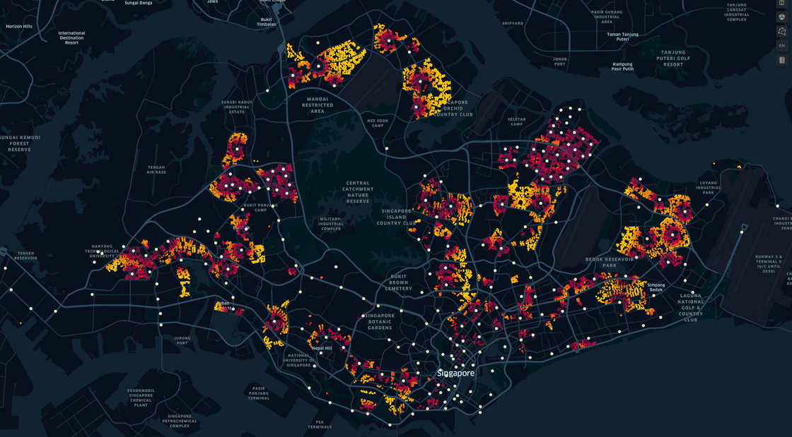
As a real estate company, we aim to better advise our clients on their property decisions. To do so, we need to have a better understanding of the property market. This project aims to ingest, process and store HDB resale data on GCP, and visualize the data using PowerBI.
One Step Further
Instead of simply downloading the data from data.gov.sg and loading a static CSV file, we decided to do the following:
- Create an automated ingestion pipeline to get the most updated data daily.
- Use the OneMap API to get the latitude and longitude of each HDB block. This allows us to plot the data on a map, and to get the nearest MRT station.
Automated Ingestion Pipeline
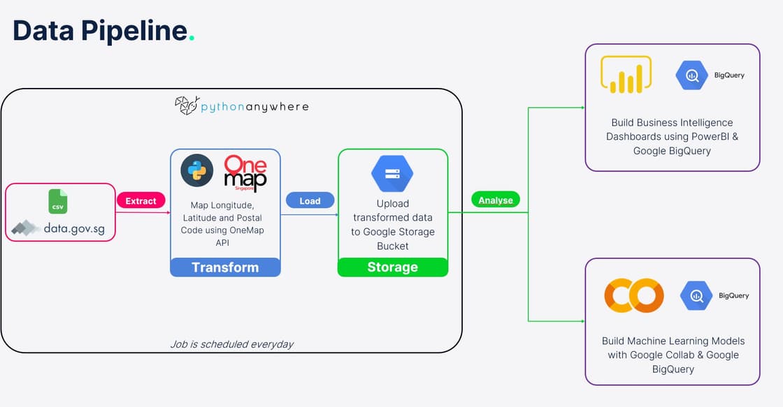
During development, the team faced a few challenges:
- Query limit of 15 rows when scraping the table from data.gov.sg.
- Initial mapping of HDB blocks to latitude and longitude took 5-6 hours, even with parallel processing due to rate limiting. (However we only need to do this once)
- Pushing the data to Google Storage Bucket required a very specific method of authentication.
- Scheduling the job to run daily.
Derived Workaround and Code
- To bypass the query limit, we modified our code to download the CSV files and performed data wrangling in Python.
- Subsequent mapping of the coordinates took about 20 - 30 seconds, as we only need to map the new blocks.
- We used a service account to authenticate the Google Storage Bucket.
- The job was deployed on PythonAnywhere, and scheduled to run daily.
1. Downloading the CSV file
def run_hdb_scrape():
    # download latest csv
    print("Downloading File..")
    download_url = "https://data.gov.sg/dataset/7a339d20-3c57-4b11-a695-9348adfd7614/download"
    response = requests.get(download_url)

    with open('resale-flat-prices.zip', 'wb') as f:
        f.write(response.content)

    # unzip the file
    with zipfile.ZipFile('resale-flat-prices.zip', 'r') as zip_ref:
        zip_ref.extractall('.')

    # delete the zip file
    os.remove('resale-flat-prices.zip')
    print("Zip file removed")

    # delete the old csv files
    filenames_to_remove = ['resale-flat-prices-based-on-approval-date-1990-1999.csv','resale-flat-prices-based-on-approval-date-2000-feb-2012.csv','resale-flat-prices-based-on-registration-date-from-jan-2015-to-dec-2016.csv','resale-flat-prices-based-on-registration-date-from-mar-2012-to-dec-2014.csv',
    'metadata-resale-flat-prices.txt'
                      ]

    for filename in filenames_to_remove:
        os.remove(filename)

    print("Files removed")

    os.rename('resale-flat-prices-based-on-registration-date-from-jan-2017-onwards.csv', 'hdb_resale_latest.csv')
2. Prepare the dataset for mapping
    # load the csv
    df_hdb_resale_latest = pd.read_csv('hdb_resale_latest.csv', low_memory=False)
    df_hdb_resale_current = pd.read_csv('hdb_resale.csv', low_memory=False)
    df_mrt_lrt = pd.read_csv('mrt_lrt_data.csv', low_memory=False)

    # create columns to match the current csv
    df_hdb_resale_latest['_id'] = df_hdb_resale_latest.index + 1
    df_hdb_resale_latest.sort_values(by=['_id'], ascending=False, inplace=True)
    df_hdb_resale_latest['Address'] = df_hdb_resale_latest['block'] + " " + df_hdb_resale_latest['street_name']

    # append to current df_resale
    df_hdb_resale_combined = pd.concat([df_hdb_resale_latest, df_hdb_resale_current])

    # drop duplicates
    df_hdb_resale_combined.drop_duplicates(subset=['_id'], keep='last', inplace=True)
3. Map the coordinates, postal code and nearest MRT station
    # Set up scraping parameters
    session = requests.Session()
    retries = Retry(total=5, backoff_factor=0.1, status_forcelist=[ 500, 502, 503, 504 ])
    session.mount('http://', HTTPAdapter(max_retries=retries))
    session.mount('https://', HTTPAdapter(max_retries=retries))

    def geocode_one_map(address):
        session = requests.Session()
        req = session.get('https://developers.onemap.sg/commonapi/search', params={'searchVal': address, 'returnGeom': 'Y', 'getAddrDetails': 'Y', 'pageNum': 1})
        resultsdict = req.json()
        if resultsdict['found'] != 0:
            lat = resultsdict['results'][0]['LATITUDE']
            lng = resultsdict['results'][0]['LONGITUDE']
            postal_code = resultsdict['results'][0]['POSTAL']
            return lat, lng, postal_code
        return None, None, None

    # Filter rows where 'Latitude' is null
    null_rows = df_hdb_resale_combined[df_hdb_resale_combined['Latitude'].isnull()]

    try:
        # Filter rows where 'Latitude' is null
        null_rows = df_hdb_resale_combined[df_hdb_resale_combined['Latitude'].isnull()]

        # Apply geocoding function to the address ('block' and 'street_name') to get latitude, longitude, and postal code
        null_rows[['Latitude', 'Longitude', 'Postal Code']] = null_rows.apply(lambda row: pd.Series(geocode_one_map(f"{row['block']} {row['street_name']}")), axis=1)

        # Tag each row to the nearest MRT/LRT Station
        for home_index, home_row in null_rows.iterrows():
            min_distance = float('inf')
            nearest_station = None

            hdb_coord = (home_row['Latitude'], home_row['Longitude'])

            for train_index, train_row in df_mrt_lrt.iterrows():
                mrt_coord = (train_row['lat'], train_row['lng'])
                distance = geodesic(hdb_coord, mrt_coord).km

                if distance < min_distance:
                    min_distance = round(distance, 2)
                    nearest_station = train_row['station_name']

            null_rows.at[home_index, 'nearest_station'] = nearest_station
            null_rows.at[home_index, 'min_distance_km'] = min_distance

        # Update the original DataFrame with the updated values
        df_hdb_resale_combined.update(null_rows)

    # if there are no null values
    except ValueError:
        pass

    print("Lat, Long, postal code, nearest MRT station & distance mapped.")
4. Clean Up
    # Convert the 'Postal Code' column to string
    df_hdb_resale_combined['Postal Code'] = df_hdb_resale_combined['Postal Code'].astype(str)
    df_hdb_resale_combined['Postal Code'] = df_hdb_resale_combined['Postal Code'].apply(lambda postal_code: postal_code.zfill(6))
    df_hdb_resale_combined.to_csv('hdb_resale.csv', index=False)
    os.remove('hdb_resale_latest.csv')
    print("Working files removed.")
5. Push to Google Storage Bucket
    # upload to google cloud storage
    print("Uploading to cloud now...")
    storage_client = storage.Client.from_service_account_json('client-secret.json')
    bucket = storage_client.bucket('hdb-resale-bucket')
    blob = bucket.blob("hdb_resale.csv")
    blob.upload_from_filename('hdb_resale.csv')
    print("HDB Resale data updated.")
Data Visualisation
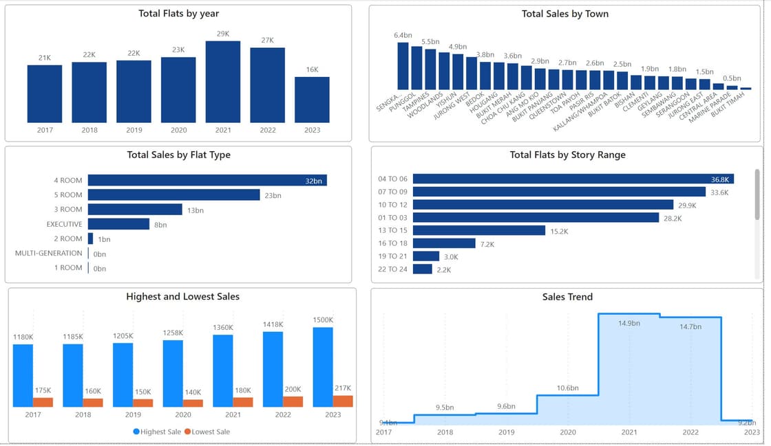
With the coordinates, we can now plot the visualisations:
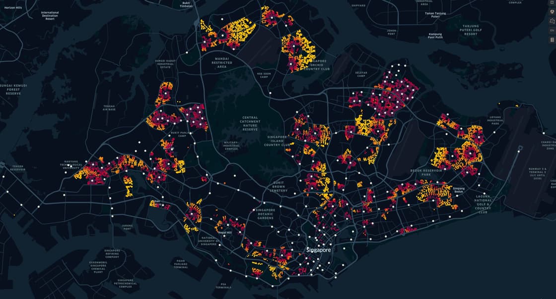
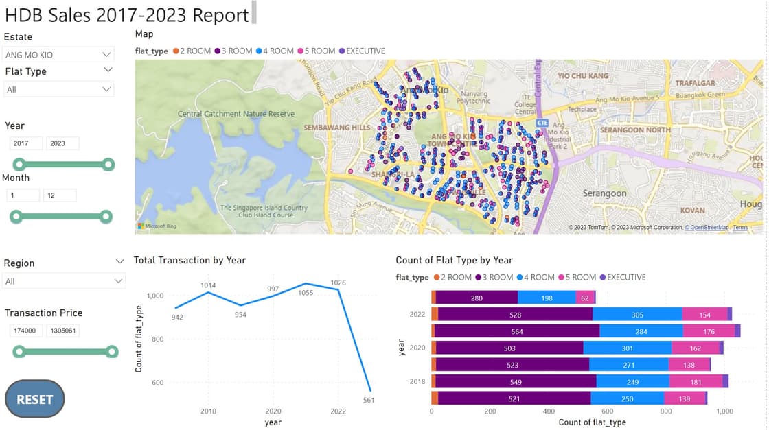
By the main landing dashboard alone, it can be inferred that URA, HDB has meticulously planned the distribution of the HDB flats, to ensure that each area has its own cluster of various flat types, with a certain ratio.
It's also interesting to point out the "herd" mentality, where resale units are usually in the same cluster, almost like a "domino effect".
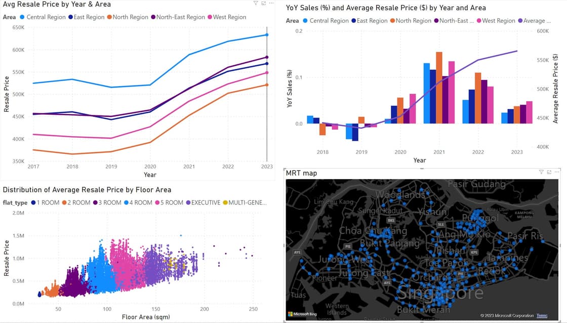
Another point worth mentioning was that the resale prices generally move in parallel, and every region follows the same trend. While the base price differs by location, the average and median price gap between each region stays roughly the same throughout 2017 – 2023.
Using the average sales, we know that:
| 2017 | 2018 | 2019 | 2020 | 2021 | 2022 | 2023 | |
|---|---|---|---|---|---|---|---|
| Central | 524,403 | 533,315 | 515,306 | 520567 | 588406 | 618428 | 633013 |
| East | 454,733 | 460,398 | 443,078 | 460115 | 513591 | 551265 | 568518 |
| North | 375,136 | 365,664 | 371,013 | 391788 | 452304 | 502011 | 519995 |
| NE | 456,614 | 453,761 | 450,072 | 464441 | 512013 | 560210 | 582892 |
| West | 409,783 | 404,422 | 401,204 | 426903 | 484261 | 522981 | 548177 |
Calculating the gap between year region for 2023, taking North as base 100% (for calculation convenience in +ve rather than -ve), we get the following:
| Central | East | NE | West | |
|---|---|---|---|---|
| Gap vs North | +21.73% | +9.33% | +5.42% | +12.09% |
A simple formula to calculate can be as such:
Predicted=Base Value+(Gap*Base Value)+(Growth Rate (*±2.25)*Base Value)
To account for the growth, we can calculate the Year-over-year (YoY) as such in PowerBI:
YoY Sales =
VAR sales_amt = [avg_sales]
VAR current_year = MAX(Query1[year])
VAR previous_sales = CALCULATE( [avg_sales], Query1[year] = current_year -1 )
VAR YoYGrowth =
    DIVIDE (
        sales_amt - previous_sales, previous_sales
    )

RETURN
IF (
    HASONEVALUE( Query1[year] ),
    IF (
        NOT ISBLANK( sales_amt ) && NOT ISBLANK( previous_sales ), YoYGrowth
    )
)
Table of YoY Sales:
| (%) | 2018 | 2019 | 2020 | 2021 | 2022 | 2023 |
|---|---|---|---|---|---|---|
| Central | +0.02 | -0.03 | +0.01 | +0.13 | +0.05 | +0.02 |
| East | +0.01 | -0.04 | +0.04 | +0.12 | +0.07 | +0.03 |
| North | -0.03 | 0.01 | +0.06 | +0.15 | +0.11 | +0.04 |
| NE | -0.01 | -0.01 | +0.03 | +0.10 | +0.09 | +0.04 |
| West | -0.01 | -0.01 | +0.06 | +0.13 | +0.08 | +0.05 |
We can now provide an estimate of the average sales for 2023:
| 2023 | 2024 (High) | 2024 (Low) | |
|---|---|---|---|
| Central | 633,013 | 656,389 | 609,590 |
| East | 568,518 | 603610 | 533,410 |
| North | 519,995 | 566,794 | 473,195 |
| NE | 582,892 | 629,661 | 536,062 |
| West | 548,177 | 606,678 | 489,679 |
Learning Points
Through this project, the team was able to observe and apply the concept of “open innovation” in practice, using real world data and examples. For example, Chesbrough noted that open innovation is essential to solve complex problems by introducing suggestions, data, ideas, or people from entirely outside of the organization (2004). In this project, the team used OneMap’s open data to map the coordinates and postal code to the HDB units.
Without the availability of such resources, it will be impossible to always get the latest data with the mapped coordinates. In an organizational context, it could cost them financial loss in terms of man-hours committed to manually mapping this data.
In the personal perspective, despite the unforeseen circumstances, I am glad that I managed to complete this project. I have learnt a lot from this project, especially on how important it is to ensure that the data is properly ingested and ready for downstream analysis. I have also applied what I learnt in Digipen on data engineering to a real-world project.